Elevation Data from Cloud-Optimized GeoTIFFs
Part 2: Color, Land Cover, and Surface Water
Introduction
Part 1 of this series introduced the U.S. Geological Survey’s Cloud-Optimized GeoTIFF (COG) data product and showed how its elevation data could be used to produce shaded-relief imagery. It also introduced the Apache Commons Imaging API, a software library that supports data access to GeoTIFF data products. So far, the techniques that I discussed were limited to the production of monochrome imagery. Adding color to a shaded-relief image allows it to convey information about climate, land cover, surface water, and other natural features.
In this article, we will explore ways of adding color to shaded-relief imagery through the use of simple elevation-based palettes as well as more realistic techniques using supplemental data sources. We will take these techniques one step at a time. The text that follows includes the following sections:
- Assigning color by elevation examines the pro's and con's of assigning color to an image strictly on the basis of elevation.
- Adding land-cover color values from a GeoTIFF shows how using an external land-cover product can improve the appearance of a shaded-relief image.
- Surface water and shapefiles discusses ways to improve the accuracy of surface water depiction by using supplemental shapefiles
- Color models illustrates the effects of applying different color models when blending colors.
- Dealing with shoreline and coastal areas offers techniques for addressing some of the problems that can arise near the transition from land to sea.
But before we get started, let’s take a look at the kind of result we can expect.
The picture below shows a color-enhanced rendering of the same San Jacinto sample area that was featured in the previous article. The sample covers a one-degree square area in Riverside County in Southern California that includes the San Jacinto Mountains, the Coachella Valley, and part of the Salton Sea. As in the previous article, all images were produced using the Commons Imaging API and the DemoCOG application. Source code for DemoCOG is available at the Gridfour software project.

The part of Southern California depicted in the image features sparse vegetation and is mostly arid though it does receive seasonal precipitation in the mountains. The distribution of snow and rainfall is clearly visible from the patches of green scattered over the higher-elevation areas. The assignment of terrestrial coloration was taken from a raster-based land-cover data set provided by the 100-Meter Natural Earth Data product (Patterson, 2020). The land-cover product will be discussed below. The surface-water features come from Shapefile (polygon) data sources downloaded from the U.S. Geological Survey National Atlas (USGS, 2020).
Assigning color by elevation
Lacking access to supplemental data sources, it is feasible to add color to a shaded-relief image strictly on the basis of elevation. To do so, we specify a palette tied to elevation intervals and apply it to the image processing. In the pictures below, I used a palette that was developed by the National Oceanographic and Atmospheric and Administration (NOAA) for its global-scale ETOPO1 elevation and bathymetry data set (NOAA, 2020). In the ETOPO1 palette, elevations at or below sea level are shown in shades of blue. Lower elevations are shown in green. And higher elevations are shown in tan or white.
As the pictures below show, the idea falls apart quickly when we compare the results to a reference source such as the Terrain view from Google Maps (Google, 2020).

There are two problems with the naïve application of a color palette. First, the traditional assignment of shades of green to low-lying regions gives a misleading impression of the land-cover. In this case, the arid, near-desert regions in the sample area are shown in a verdant green tone that implies abundant vegetation. Second, the fact that a large portion of the San Jacinto sample area lies below Mean Sea Level (MSL) results in dry land being colored in shades of blue. Consequently, much of the arid Coachella Valley appears to be covered with water. If the rendering were to be believed, the town of Coachella itself, which lies at 21 meters below sea level, would be entirely submerged.
Of course, it is possible to adjust the palette so that the water colors start at a lower elevation. For the panel below on the right, I tweaked the intervals so that the blue colors started at 70.1 meters below MSL. That value produces a blue area that matches the shoreline of the Salton Sea, a well-known saltwater lake. It can be interpreted as the elevation of the surface of that body of water. But the elevation of 70.1 meters below MSL does not agree with any published value for the surface of the Salton Sea that I was able to find. The value I used was obtained through several rounds of trial and error.
So, as the panel shows, a custom palette can help improve the accuracy of a color-coded elevation rendering. But, while creating a palette to fit a particular sample area is feasible, it is tedious at best and still prone to error. It also fails to capture any lakes or reservoirs that may occur at higher elevations. For that purpose, we need additional data sources such as the surface-water Shapefiles that will be discussed below.

Adding land-cover color values from a GeoTIFF
Let's see what we can do to improve the depiction of the San Jacinto data sample. The first thing we’re going to take care of is the depiction of land-cover. To that end, we turn to Tom Patterson’s Natural Earth Map Data collections. Mr. Patterson’s work is extraordinary both for its technical merit and for his generosity in offering it free-of-charge and in the public domain. There are actually two Natural Earth products. The primary Natural Earth Data website includes land-cover GeoTIFF images for the whole Earth at a moderate resolution (Natural Earth Data, 2020). But there is also a larger scale set of images giving land-cover for the United States at a 100-meter resolution at Mr. Patterson's website http://shadedrelief.com/NE_100m/. We will use this higher resolution product because it is closer to the map scale used for the elevation data in the Cloud-Optimized GeoTIFF products.
The land-cover imagery is a much different kind of GeoTIFF than the USGS elevation product that we discussed in Part 1 of this series. For one thing, it includes a conventional RGB image product rather than numerical elevation data. It also uses a Projected Coordinate System (PCS) rather than the Geographic Coordinate System (GCS) used by the USGS products. In a projected coordinate system, the pixels represent positions on the Earth that are transformed to an imaging plane using a map projection. The advantage to this approach is that the projected image can preserve important features such as area, distance, or shape that are not well represented by geographic coordinate systems.
You may recall that for the elevation data set we used in Part 1, we needed to narrow the image area in order to preserve the shape of features on the surface of the Earth. A projected coordinate system does the same kind of thing, but it does it using a much more accurate (and complex) transformation.
Let’s look briefly at the content of the GeoKeyDirectoryTag for the file W_CONUS_100m_NE_LC.tif
     key     ref     len   value/pos
       1       1       0       8   version
    1024       0       1       1   GtModelTypeGeoKey -- 1 means projected
    1025       0       1       1   GtRasterTypeGeoKey --  PixelIsArea
    1026   34737      21       0   GtCitationGeoKey – descriptive text
    2049   34737      12      21   GeodeticCitatonGeoKey – descriptive text
    2054       0       1    9102   GeogAngularUnitsGeoKey -- 9102 means degrees
    2062   34736       3       0   TOWGS84GeoKey  -- “To WGS84” transformation data
    3072       0       1    5070   ProjectedCRSGeoKey – refers to EPSG 5070
    3076       0       1    9001   ProjLinearUnitsGeoKey    (linear meter)
In this data set, key 1024 (GtModelTypeKey) has the value 1, indicating that the GeoTIFF uses a projected coordinate system. Key 3072 (projected coordinate reference system geo key) refers to the European Petroleum Survey Group (EPSG) map projection database specification number 5070 (EPSG, 2020). Although this particular GeoTIFF does not give a full set of parameters for the map projection it uses, we can look it up the necessary elements from external sources. The ESPG system is well known and its specifications are readily available on the Internet. ESPG map projection 5070 is an Albers Equal Area Conic map projection optimized for depicting features in the Contiguous United States (CONUS).
The fact that the substantial majority of GIS analysis is conducted using a projected coordinate system is not due to a love of complexity. Rather, it is because working on a plane-based coordinate system is so much easier than performing analysis over the surface of the spheroidal Earth. Transforming coordinates onto a projected plane simplifies the mathematics for geospatial computations (area, distance, and angle) and also transforms features into a form that is visually closer to their real-world counterparts. The downside to this approach is that because the Natural Earth Land-Cover data set uses a projected coordinate system, we need an implementation of a map projection in order to correlate the geographic coordinates from the Cloud Optimized GeoTIFFs with the pixel positions in the land-cover image.
In the previous article, we discussed how the GeoTIFF metadata allowed us to transform the raster coordinates from the source data to geographic (latitude, longitude) coordinates and permitted the data to be registered with real-world locations. That coordinate conversion was accomplished using a simple scale and offset transformation (an affine transformation). To register the elevation with the land-cover GeoTIFF, we need to perform two more transformations. First we need to map geographic coordinates to the map projection coordinate system defined by the land-cover GeoTIFF. Then we need to use an affine transformation to scale and offset the projected coordinates to the raster coordinate system. Once we have mapped coordinates from the raster elevation product to the corresponding raster coordinates for Natural Earth GeoTIFF, we can access the pixels in the land-cover imagery to find the color values associated with each elevation grid cell. The transformation chain is summarized below.

For the DemoCOG implementation, I elected to write my own implementation of the Albers Equal Area Conic map projection used by the Natural Earth GeoTIFF. While general purpose map-projection APIs are available on the web, I didn’t want to add yet another software dependency to the demonstration application. So I wrote a single class to perform the forward transform (geographic to projected) that the demonstration application required. Fortunately, the Albers is not very complicated as map projections go. Formulas for the transformation are given in John P. Snyder’s classic book “Map projections – a working manual” (Snyder, 1987). Although coding Mr. Snyder’s formulas required care, it was not difficult.
The full size of the Natural Earth Land-Cover GeoTIFF for the western half of the United States is quite large, 25403 by 31390 pixels. Fortunately, the Commons Imaging API allows us to access just the subset of the image that we actually need. So, loading the land-cover imagery associated with the area of interest for our shaded-relief image is just a matter of using the following steps:
- Using the Albers Equal Area map projection, transform the geographic coordinates for the four corners of the San Jacinto data product to pixel coordinates in the land-cover imagery.
- Use the pixel coordinates to determine the bounds of the sub image required for rendering.
- Load the sub image.
- For each raster cell in the shaded-relief image:
- Find the geographic coordinates of the raster cell
- Map the geographic coordinates to pixel coordinates in the land-cover sub image (because the elevation data set has 10-meter spacing while the land-cover data set has 100-meter spacing, this result will be a fractional value, often falling between pixels).
- Interpolate the color values for the output pixel coordinates.
- Apply the color to the shaded-relief imagery.
The picture below shows the raw image extracted from the Land-Cover GeoTIFF (left) and the result when the image is combined with shaded-relief data created from the USGS elevation data set. One natural phenomenon that the Natural Earth Land-Cover image doesn’t depict is surface water. We will discuss technique for adding that information next.

Surface water and shapefiles
You may be wondering why Mr. Patterson decided to omit surface water from his land-cover imagery. It turns out that removing surface-water features allows application to use alternate data sources that can provide better results. The 100-meter pixel spacing for the Natural Earth GeoTIFF is adequate for land-cover. But most surface water features included on maps are drawn at a much higher resolution than that. Omitting surface water from the Land-Cover depiction leaves developers and cartographers free to use other sources. And, because surface water data in the form of Shapefile (polygon) data products is easy to come by, omitting it from a land-cover product is not an obstacle for its users. Mr. Patterson himself recommends surface water Shapefile products from the USGS National Atlas (USGS, 2020).
A Shapefile is an industry standard GIS data format that represents an area-based feature such as lake as a polygon defined by a series of using spatial coordinates that define its vertices. For this article, Shapefiles from the National Atlas were downloaded from the Earth Explorer website (USGS, 2020). To extract data from these files for rendering, the demonstration application uses an API from the open-source Tinfour software product (Tinfour, 2020). The results were shown in the larger-scale image that introduced this article.
Color models
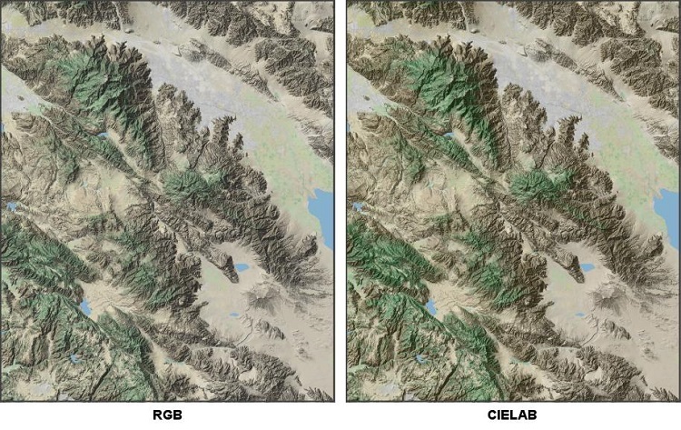
The Natural Earth Land-Cover GeoTIFF uses a conventional RGB (Red-Green-Blue) color model. If you look through the DemoCOG code, you may be surprised by the complexity of the color processing used to interpolate those RGB values to populate the output image. The DemoCOG application uses an alternate color model known as CIELAB (“CIELAB color space”, Wikipedia, n.d.). While the RGB color model is well suited for the implementation of computer monitors and display hardware, the CIELAB model is a closer match for the way the human eye perceives color. Thus the CIELAB model can produce better results when blending colors. The Apache Commons Imaging API includes a set of utilities for converting between the RGB color space (which is used by the source image and output display) and the CIELAB model. The DemoCOG application takes advantage of these conversions for its color manipulation and processing.
That being said, I do not wish to overstate the case for using the alternate CIELAB model rather than working directly from RGB. The color palette used to the Natural Earth Land-Cover imagery works well in both systems. As the panels below show, the CIELAB treatment produces somewhat richer colors and enhanced contrast. But the differences are subtle.
Dealing with shoreline and coastal areas
Although the San Jacinto data set includes a number of interesting features, it lies well inland and does not include shoreline or ocean areas. For an example of an area that includes coastal waters, we turn to another Cloud Optimized GeoTIFF downloaded from the USGS. The image below was constructed from data for an area that covers Western Connecticut and a section of Southeastern New York State. It includes the U.S. Military Academy at West Point, the town of Sleepy Hollow in New York, the Connecticut cities of Norwalk, Danbury and Waterbury, as well as Lake Candlewood and numerous other lakes and rivers. The blue strip on the left side of the image is the Hudson River.
New York and Connecticut receive reasonably regular rainfall and snow. Consequently, the land-cover depiction is much greener than for the area near the San Jacinto mountain range. The Northeast U.S. area shown above is also much more urbanized than the San Jacinto area. The Natural Earth Land Cover data set uses gray tints to show built-up areas, so most of the coastal area from Connecticut is drawn in gray.
Geologically, the Western Connecticut sample area is much older than the San Jacinto area. Its hilly terrain is the result of millions of years of weathering and was significantly modified by glaciation during the ice age. Some of the effects of that modification are revealed by the shaded-relief rendering, most notably the shaping of the north-south orientated ridges and valleys across the region.

The coverage of the Natural Earth Land-Cover imagery does not extend into the ocean area. Where the land-cover information ends, the tint imagery supplies white pixel values. In most cases, the DemoCOG application assigns output pixels a blue color where elevations lie at or below sea level. But because of the elevation raster has so much greater resolution than the land-cover imagery, there are occasional conflicts in the data. Sometimes, pixels with elevations indicating that they should be land positions happen to fall over the white area in the Natural Earth product. Because they are identified as land pixels, the rendering application would ordinarily take the color value from Natural Earth. But if it were to do so, the result would be a speckling of white pixels along the shore line as shown in the panels below. To correct for such cases, DemoCOG implements logic to extend land tints outward from the coastline.

Conclusion
The U.S. Geological Survey’s Cloud Optimized GeoTIFF (COG) products provide a valuable source of high-resolution elevation data that can be downloaded free-of-charge. There are many potential applications for the USGS elevation data. This article focuses on one of them: the creation of shaded-relief map imagery.
Discussing shaded-relief imagery gave us an opportunity to explore the underlying concepts used in GeoTIFF files. It also gave us an opportunity to exercise some of these concepts through the implementation of a data access and map rendering tool called DemoCOG.
DemoCOG uses the Apache Commons Imaging software library to access GeoTIFF files and obtain the three fundamental data elements necessary to perform shaded-relief rendering: raster-based elevation data, geolocation metadata, and georeferenced imagery (the Natural Earth land-cover information). Commons Imaging also provided the color-space conversion tools that allowed DemoCOG to perform optimal color-blending and interpolation operations. The source code for the DemoCOG application is available from the Gridfour Software Project. Although DemoCOG is implemented in the Java programming language, its code includes plenty of comments and is written to be accessible to readers who are unfamiliar with Java.
I hope you’ve found this series of articles useful. Although the GeoTIFF format can seem overwhelmingly complex at first, it is based on a logical series of design choices that make it manageable once you delve into it. I wish you success in working with GeoTIFF products and the Apache Commons Image software library.
References
CIELAB color space. (n.d.). In Wikipedia Retrieved July 2020 from https://en.wikipedia.org/wiki/CIELAB_color_space.
Google. (2020). Google Maps. Accessed September 2020 from https://www.google.com/maps/@33.4231449,-116.2146336,10z/data=!5m1!1e4
Natural Earth Data. (2020). Natural Earth – Free vector and raster map data at 1:10m, 1:50m, and 1:110m scales. Retrieved June 2020 from https://www.naturalearthdata.com/
Open Geospatial Consortium [OGC]. (2019). OGC GeoTIFF Standard. Accessed May 2020 from http://docs.opengeospatial.org/is/19-008r4/19-008r4.html. See also PDF document accessed May 2020 from https://cdn.earthdata.nasa.gov/conduit/upload/12428/19-008r4.pdf
Patterson, Tom. (2020). 100-meter Natural Earth Map Data. Retrieved May 2020 from http://shadedrelief.com/NE_100m/
Snyder, John. (1987). Map projections – a working manual. U.S. Geological Survey professional paper; 1935. Retrieved April, 2020 from https://pubs.usgs.gov/pp/1395/report.pdf
Tinfour. (2020). The Tinfour Software Project. Accessed May 2020 from http://tinfour.org
Data sources
The USGS Cloud Optimized GeoTIFF elevation data sources are located at the following sites:
- Via FTP: ftp://rockyftp.cr.usgs.gov/vdelivery/Datasets/Staged/Elevation/13/TIFF/
- Via HTML (Amazon cloud) http://prd-tnm.s3.amazonaws.com/index.html?prefix=StagedProducts/Elevation/13/TIFF/
Shapefiles providing coastlines, surface-water features, political boundaries, etc. are available from the U.S. Geological Survey (USGS) EarthExplorer website. Data at a map scale of 1:1 million that was collected for the discontinued U.S. National Atlas may be downloaded using using the following procedure that is taken from Tom Patterson's Shaded Relief website:
Click the "Data Sets" tab then select Digital Maps/National Atlas. Then click the "Additional Criteria" tab and specify Collection/1:1,000,000-scale before clicking the "Results" button in the lower right (Patterson, 2020).
Shapefiles and land-cover GeoTIFFs providing data for the entire Earth at 1:10 million scale is available at the Natural Earth website.