This article is under construction. Additional content and editorial improvements are coming soon.

Note: The 2D Delaunay triangulation is the focus of the Tinfour Software Project. Background information on the Delaunay is available from the Tinfour project document An introduction to the Delaunay triangulation.

Introduction

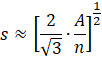
The Delaunay triangulation is a useful technique for evaluating the distances between neighboring samples in a set of unstructured data points. In cases where the data points are distributed with a uniform density across a surface, we can estimate the average spacing between neighboring samples, s, using a simple calculation, , where A is the area of a polygon containing n samples (see below). But, in cases where the point spacing is non-uniform, the simple calculation may be insufficient. To compute actual distances between points in a set with local variations in density, we need a method for establishing which pairs of samples can be treated as neighbors. The Delaunay triangulation provides one such method.

For most applications, the goal of the 2D Delaunay is to build a triangle-based mesh from a set of points distributed over a surface. In the course of constructing the mesh, the process links pairs of points based on the Delaunay criterion (Lucas, 2016). This selection technique guarantees that the resulting set of triangles is optimal in many regards. Although the Delaunay optimization is focused on the structure of its triangles rather than the assignment of neighbors, the resulting selection of neighboring vertex pairs does provide a good balance between proximity, directionality, and density. As such, the Delaunay triangulation provides a reliable technique for identifying which samples are treated neighbors and can be used to compute sample spacing.

Preliminaries

To see how the Delaunay triangulation is used to identify neighboring sample pairs, we will take a look at a few underlying ideas for the technique. Specific issues in using the Delaunay will be discussed in the section Applying the Delaunay to a sample spacing calculation below.

The uniform density case

In the special case where samples are distributed across the surface with a nearly uniform density, we can compute the point spacing using the formula introduced above. This formula is derived by approximating the sample set with a truly uniform point distribution. When all points are equally spaced on the plane, they form a tessellation consisting of equilateral triangles. An example is as shown in the figure below.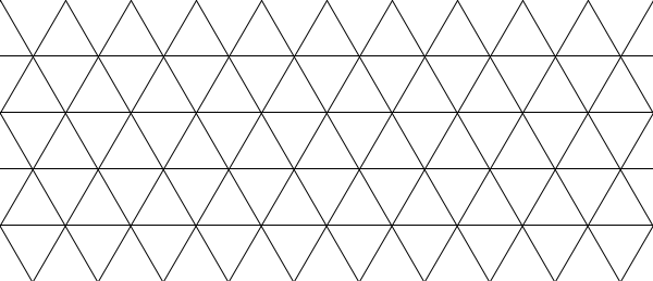

We wish to find the uniform distance between points, s, which is also the length of the sides of the triangles in the tessellation For a sufficiently large number of points, n, the number of triangles in the tessellation covering a bounded area approaches 2n. The area of each equilateral triangles is . So, given the area A of the bounded region containing the sample points, we have

and, solving for s:

which gives us our approximation .

Incidentally, the uniform tessellation shown in the figure above happens to be a Delaunay triangulation. So the Delaumay-based techniques that works for a collection of non-uniformly spaced samples also applies to the uniform and nearly uniform cases.

The Delaunay criterion

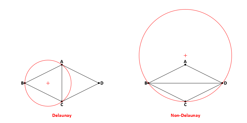
A Delaunay triangulation links pairs of sample points to form triangles that conform to the Delaunay criterion. The criterion itself is based on the idea that if we were to construct a circumcircle from the three vertices of the triangle, no other vertices in the triangulation would lie within the closed bounds of the circumcircle.

The key to constructing a conforming triangulation is to ensure that we choose which vertices to link in such a way that the triangles that they form do not violate the Delaunay criterion. Referring to the figure below, we see that the circumcircle for triangle ABC does not include vertex D. So the triangulation on the left is properly Delaunay. Alternatively, if we were to link vertices B and D, to form triangle BCD, the resulting circumcircle would enclose vertex A. So the triangulation on the right is not properly Delaunay. A proof from geometry shows that if we have two adjacent triangles, such as ABC and ACD, if one triangle is Delaunay conforming, them both are Delaunay conforming.

There are a number of algorithms for constructing a Delaunay triangulation. In all cases, though, the result is that the circumcircle for each triangle does not enclose any other point from the sample set. A Delaunay triangulation has a number of desirable properties. For our purposes, we will consider the following which were described by Mount (2020):

1. Closest pair property: The closest pairs of vertices in a Delaunay triangulation are neighbors.
2. Average minimum angle property: Among all feasible triangulations, the Delaunay maximizes the minimum average angle. Thus, the Delaunay tends to avoid skinny triangles.

The closest pair property tells us that the Delaunay supports the common-sense idea that a sample is always treated as the neighbor of the sample that lies closest to it. For our purposes, that characteristic is reassuring. The second property tells us that the Delaunay tends to form a set of triangles that are as robust as possible (i.e. will have as a large a minimum angle as possible). The most robust case of a triangle is the equilateral, such as the ones that were shown in the uniform density tessellation shown in Figure 1 above. So the fact that the Delaunay process attempts to create robust triangles suggests that the mesh it produces will be as close to a uniform density as is feasible for a set of points.

The Delaunay triangulation with non-uniform spacing

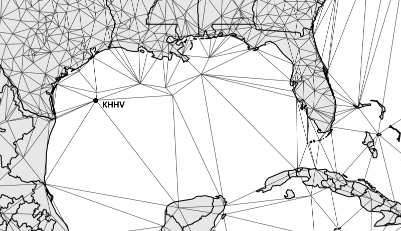
The figure below shows an example of a Delaunay triangulation constructed for the locations of weather-reporting stations located in the area of the Gulf of Mexico. Most of the stations are located at scattered positions on land, though a few are located over the water. The sample labeled KHHV is an automated reporting station based on an oil drilling platform. As noted above, the closest pair property ensures that the Delaunay links KHHV to its nearest neighbor, a station located immediately to its north. As the image shows, many land-based stations to the north and west are not treated as linked neighbors even though they are relatively close to KHHV. On the other hand, a station to its southwest on the Yucatan Peninsula is treated as a neighbor even though it is relatively far away from KHHV. This example illustrates the way the Delaunay based neighbor selection does not depend on a simple distance calculation, but adapts to the general spacing of the samples in all directions.

Applying the Delaunay to a sample spacing calculation

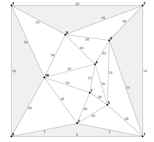
Most software packages that construct a Delaunay triangulation include some method for iterating through its component edges. There is, however, one complication when using the lengths of edges in the Delaunay triangulation as a way of evaluating sample spacing. Some of the edges near the perimeter of the triangulation do not follow the same rules as those in the interior.

The figure below shows a case where the perimeter edges are much longer than those in the interior. That happens because there are no points located outside of the Delaunay triangulation. When we discussed the Delaunay criterion above, we noted that the decision for linking an edge depended on the placement of vertices on either side of the edge. But, because there are no points beyond the perimeter edges, the resulting triangles cannot be evaluated for compliance with the Delaunay criterion. They are independent of it. They do not violate the criterion, but neither do they support it.

In tabulating the distances between points in a Delaunay triangulation, it is useful to omit those triangles that are associated with exterior edges. Looking at the upper left of the figure, we see that the perimeter edge from vertex 4 down to vertex 0 is labled with edge-index 18. Edge 18 forms a triangle using vertex 10 with edges 58 and 10. Because the triangle with vertices 4, 0, and 10 is not strictly Delaunay conforming, we exclude its three edges (18, 58, and 10) from the sample-distance tabulation.

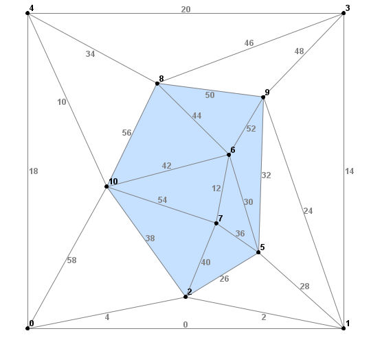
In the figure below, the area shown in light blue includes the edges that would be added to the tabulation. Due to the relatively small sample size, almost half of the edges in the triangulation were excluded from the tabulation. For large sample sizes, the number of edges associated with the perimeter is much smaller than those associated with the interior.

Constraint edges

In some cases, a software application that uses a Delaunay triangulation may specify constraints on the way edges are constructed. When that happens, some of the resulting edges may be non-Delaunay. When tabulating sample spacing for constrained Delaunay triangulations, constraint edges are generally treated the same way as the perimeter edges described above. For more information on the use of constraints in the Delaunay, see the Tinfour article
What is the constrained Delaunay trianglation and why would you care?

A real-world example

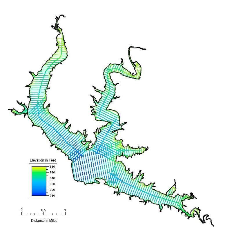
Let's take a look at a real-world data set and compare how sample spacing computed using the Delaunay method compares to specifications provided by the data's publisher. The figure below shows a map of the Lake of the Arbuckles, an artificial reservoir located in Murray County, Oklahoma, USA. In 2016, the Oklahoma Water Resources Board (OWRB) conducted a bathymetric survey of the lake (OWRB, 2016). The survey used a boat equipped with sonar device to record bottom depth samples. The boat followed a pre-planned path and collected data at intervals of 5 feet (1.5 meters) along the survey tracks. By design, the tracks are separated by 250 feet (76 meters). Because the distance between samples is so small compared to the scale of the map, the point positions in the figure often overlap and the tracks appear as solid lines.

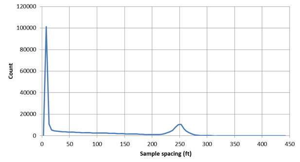
Based on the information provided by the data publisher, we expect the distribution of sample spacing to fall into two groups: the distances between samples along each track, and the distances between tracks. By processing the data using the Delaunay technique, we obtained the graph below. The graph shows how many times we encountered a sample space with a particular value. As expected, there is a peak corresponding to the 5-foot interval along the track and a smaller bump for the 250 foot distance between tracks.

Conclusion

To evaluate the distances between samples in a point-value data set, we need a method of determining which pairs of samples can be treated as neighbors. The properties of the Delaunay triangulation make it a good tool for that purpose. Several implementations of the Delaunay triangulation exist on the Internet. The examples provided in these notes were created using a Java-based implementation of the Delaunay triangulation which is available from the Tinfour Software Project. A C# version of Tinfour is available from Tinfour.NET.

References

Lucas, G. (2016). An introduction to the Delaunay triangulation.
https://gwlucastrig.github.io/TinfourDocs/DelaunayIntro/index.html/

Mount, D. (2020). CMSC 754: Lecture 12 -- Delaunay triangulations: general properties [PDF].
https://www.cs.umd.edu/class/spring2020/cmsc754/Lects/lect12-delaun-prop.pdf

Oklahoma Water Resources Board [OWRB]. (2016). Bathymetric Survey of Select Dissolved Oxygen Impaired Reservoirs. Final Report July 1, 2016 [PDF].
https://oklahoma.gov/content/dam/ok/en/owrb/documents/maps-and-data/bathymetric-surveys/FY2016%20DO%20Mitigation%20Bathy%20Mapping%20Report-Final%20Report.pdf"